第3回：遺伝的アルゴリズム（GA）で巡回セールスマン問題（TSP）を解く

0. 第3回の到達目標¶

第3回終了時に、次を説明・実装のイメージまで持てる状態を目指す。

TSP を 順列（permutation；巡回順・ツアー） としてモデル化し、 目的関数（objective function） （総距離）を定義できる。
第2回：binary GA による特徴選択（SVM × 手書き数字認識） §2 の内容と整合する形で、GA の 遺伝的操作 と 個体集団 $P(t)$ の更新を説明できる。
TSP において 順序を保つ交叉（order-preserving crossover） （順序交叉など）が必要な理由を説明できる。
パラメータ（ 個体数（population size） 、 世代数（number of generations） 、 交叉率（crossover rate） 、 突然変異率（mutation rate） 、 エリート数（elite count） ）が結果に与える影響を定性的に述べられる。

1. 本日の位置づけ（第1回との接続）¶

第1回では次を整理した。

組合せ最適化では解候補が膨大になり、全探索が非現実的になりやすい。
メタヒューリスティクス（metaheuristics） は、汎用的な探索の枠組みとして近似解を求める。

本日は 巡回セールスマン問題（TSP: Traveling Salesman Problem） に 遺伝的アルゴリズム（GA） を適用する。GA の一般論は第2回：binary GA による特徴選択（SVM × 手書き数字認識）で扱い、本資料では 順列染色体と順序交叉 など TSP 固有の点に絞って補足する。

2. TSP の定式化（復習）¶

2.1 問題の言い換え¶

$n$ 個の都市（地点）があり、各都市はちょうど1回ずつ訪問する。
出発都市に戻る 閉路（closed tour / Hamiltonian cycle） とする（ここではこの形を扱う）。
隣接都市間の 距離（distance） または 移動コスト（travel cost） が与えられる。
総移動距離（総コスト）を最小化（minimize） する巡回順序を求める。

2.2 解の表現¶

都市に $0, 1, \ldots, n-1$ の番号を付ける。
解は 都市番号の順列 $\pi = (\pi_0, \pi_1, \ldots, \pi_{n-1})$ で表す。

$\pi_k$ : $k$ 番目に訪問する都市の番号（順列を 染色体（chromosome） とみなすとき、各位置の値を 遺伝子（gene） と呼ぶ）
順列であること自体が「各都市を一度ずつ訪れる」という 制約（constraint） を表す
ここでは染色体と巡回順序（ 表現型（phenotype） ）を同一視して扱う（ 遺伝子型（genotype） と区別しない簡略モデル）

2.3 目的関数（評価値）¶

2次元座標 $(x_i, y_i)$ が与えられる場合、 ユークリッド距離（Euclidean distance） を用いることが多い。

d(i, j) = \sqrt{(x_i - x_j)^2 + (y_i - y_j)^2}

(1)

総距離（最小化したい量）は次である。

L(\pi) = \sum_{k=0}^{n-2} d(\pi_k, \pi_{k+1}) + d(\pi_{n-1}, \pi_0)

(2)

無向グラフとして与えられる場合¶

都市を 頂点（vertex；ノード node） とみなし、都市間の移動コストを 無向辺の重み（undirected edge weight） として与えた 無向グラフ（undirected graph） $G=(V,E)$ が与えられる場合もある。
頂点集合 $V$ の各要素が都市に対応し、辺 $\{i,j\} \in E$ には非負の重み $w_{ij}=w_{ji}$ が付く（ 完全グラフ（complete graph） であれば、任意の都市の組に辺があり、どの順序でも巡回できる）。

このとき、巡回順 $\pi$ に沿った総コストは、辺の重みの和として次で与えられる。

L(\pi) = \sum_{k=0}^{n-2} w_{\pi_k,\pi_{k+1}} + w_{\pi_{n-1},\pi_0}

(3)

各都市対がユークリッド距離 $d(i,j)$ で結ばれる完全無向グラフとみなすと $w_{ij}=d(i,j)$ となり、上の座標による定義と一致する。

個体（individual） $i$ の染色体に対応する巡回を $\pi^{(i)}$ と書く。 目的関数値（objective value） は $L(\pi^{(i)})$ である。
参考資料と同様に 適応度（fitness） を $g_i$ と書く場合、 最大化（maximization） する GA では $g_i$ が大きいほど良い個体となる。
TSP のように 最小化（minimization） する場合は、例えば $g_i = 1 / L(\pi^{(i)})$ や $g_i = -L(\pi^{(i)})$ など、 $g_i$ が良い解ほど大きくなるように定めてから 選択（selection） に用いる（実装で min を直接使っても、概念上は適応度に読み替えられる）。

3. GA の一般論と本資料（TSP）で足りる説明¶

3.1 binary GA ノートに任せる部分¶

用語（個体・適応度・選択・交叉・突然変異・世代交代）、世代の流れ、ルーレットを想定したブロック図、および 実装チェックリストの骨格は、第2回：binary GA による特徴選択（SVM × 手書き数字認識）の §2 にまとめてある。まずそちらを読み、本資料では TSP＝順列符号化 に特有の差分だけを補う。

3.2 TSP で異なる点（ここだけ押さえる）¶

符号化：染色体は 都市番号の順列 $\pi$ である（§2）。binary ノートのビット列とは異なり、順列制約（各都市ちょうど1回）が構造として埋め込まれる。
目的と適応度：最小化したいのは総距離 $L(\pi)$ である（§2.3）。GA の選択は 最大化の適応度 と整合させるため、例えば $g = 1/L$ や $g = -L$ としてから トーナメント や ルーレット に渡す（実装で min を直接追ってもよい）。
交叉：区間を切り貼りする 一点交叉・一様交叉 をそのまま使うと、子に 都市の重複・欠落 が生じやすい。TSP では 順序交叉（OX） や PMX など 順序を保つ交叉 が必要である（§4.4）。
突然変異：ビット反転の代わりに、2 位置の スワップ や 区間逆転 など、順列を保つ近傍操作 が典型である（§4.5）。

以上を除き、 $P(t)$ の更新の枠組み（評価→選択→交叉→突然変異→エリートと世代交代）は binary ノートと同じ考え方である。

4. TSP における GA の設計（binary ノート §2.2 の TSP 版）¶

第2回：binary GA による特徴選択（SVM × 手書き数字認識） §2.2 のチェックリストと 同じ順序 で、TSP（順列染色体）のときの 初期化・評価・選択・交叉・突然変異・世代交代 の要点をまとめる。実装するときは、この章を上から順に読みながら各関数を対応づけるとよい。

各節の Python の例 は学習用の断片である。必要な import（標準ライブラリの typing、サードパーティの matplotlib と numpy）は §4.1 の最初のコードブロックに一度だけ 示す。以降の各節のブロックでは import を繰り返さない。1つのスクリプトにまとめるときも同様に先頭へ集約し、 関数の定義順 （後の節が前の節の関数を呼ぶ場合は、被依存側を上に置く）を調整すること。 NumPy の ndarray と numpy.random.Generator を用い、座標・集団・距離の計算をベクトル化する。

4.1 ステップ1：初期個体群の生成（initialization）¶

都市の座標（または距離行列）を用意し、問題インスタンスを定める。
個体数（population size） $M$ 個の 順列（permutation） を、重複のない巡回順になるよう ランダムに生成 し、初期集団 $P(0)$ とする。
乱数の シード（seed） を固定しておくと、結果の再現やデバッグがしやすい。

あらかじめ、訪れる都市に番号を振っていると考えてください。このノートブックでは，各個体が持っている染色体は，その中のそれぞれの遺伝子が都市番号そのものです．染色体配列の先頭から数字を読んでいけば，それがそのままセールスマンが訪れる都市の順番になります．

このコーディング方法は，都市の巡回順番を可視化する際に便利です．一方で，交叉の実装が多少複雑になります（これは個人的感想です）．

from typing import Optional

import matplotlib.pyplot as plt
import numpy as np


def random_city_coords(
    n: int, xmax: int, ymax: int, rng: np.random.Generator
) -> np.ndarray:
    """整数範囲内に n 都市の 2 次元座標を乱数で生成する。

    Args:
        n: 都市数。
        xmax: x 座標の最大値（0 以上 xmax 以下の整数）。
        ymax: y 座標の最大値（0 以上 ymax 以下の整数）。
        rng: NumPy の擬似乱数ジェネレータ。

    Returns:
        形状 ``(n, 2)`` の float64 配列。各行が都市の ``(x, y)`` 。
    """
    x = rng.integers(0, xmax + 1, size=n)
    y = rng.integers(0, ymax + 1, size=n)
    return np.column_stack([x, y]).astype(np.float64)


def random_permutation(n: int, rng: np.random.Generator) -> np.ndarray:
    """TSP 用の1本の染色体（0..n-1 の順列）を生成する。

    Args:
        n: 都市数（遺伝子長）。
        rng: NumPy の擬似乱数ジェネレータ。

    Returns:
        形状 ``(n,)`` の int64 配列。都市インデックスの順列。
    """
    return rng.permutation(n).astype(np.int64)


def initial_population(
    pop_size: int, n: int, rng: np.random.Generator
) -> np.ndarray:
    """初期集団 ``P(0)`` をランダム順列で構築する。

    Args:
        pop_size: 個体数。
        n: 1 個体あたりの遺伝子長（都市数）。
        rng: NumPy の擬似乱数ジェネレータ。

    Returns:
        形状 ``(pop_size, n)`` の int64 配列。各行が1個体の順列。
    """
    rows = [random_permutation(n, rng) for _ in range(pop_size)]
    return np.stack(rows, axis=0)


def normalize_route_start(route: np.ndarray, start_city: int) -> np.ndarray:
    """順列を回転して ``start_city`` を必ず先頭に置く。

    Args:
        route: 都市インデックスの順列。形状 ``(n,)`` 。
        start_city: 始点として固定する都市番号。

    Returns:
        ``start_city`` が先頭に来るように回転した順列のコピー。
    """
    pos = int(np.where(route == start_city)[0][0])
    return np.roll(route, -pos).astype(np.int64, copy=False)


def normalize_population_start(
    population: np.ndarray, start_city: int
) -> np.ndarray:
    """集団の全個体に ``normalize_route_start`` を適用する。

    Args:
        population: 形状 ``(pop_size, n)`` の順列集団。
        start_city: 始点として固定する都市番号。

    Returns:
        全個体が ``start_city`` 始まりになった新しい配列。
    """
    rows = [normalize_route_start(route, start_city) for route in population]
    return np.stack(rows, axis=0)


# 例: 再現性のためビットジェネレータにシードを渡す
rng = np.random.default_rng(42)
coords = random_city_coords(8, 200, 200, rng)
population = initial_population(pop_size=30, n=coords.shape[0], rng=rng)
population = normalize_population_start(population, start_city=0)

4.2 ステップ2：評価（evaluation；適応度の計算）¶

各個体の染色体（巡回順）に対し、§2.3 の 目的関数値（objective value） $L(\pi)$ を計算する。
最小化 の GA で選択に使う場合は、 $L$ から 適応度（fitness） $g_i$ を「大きいほど良い」ように定める（例: $g_i = 1/L$ 、 $g_i = -L$ ）。
距離行列やグラフ重みを保持しておくと、評価のたびに同じ計算を簡潔に書ける。

def tour_length(route: np.ndarray, coords: np.ndarray) -> float:
    """1 個体の閉路ツアー長（ユークリッド距離の和）を計算する。

    Args:
        route: 訪問順。形状 ``(n,)`` の都市インデックスの順列。
        coords: 都市座標。形状 ``(n, 2)`` 。

    Returns:
        出発都市へ戻る閉路の総距離（スカラー）。
    """
    pts = coords[route.astype(np.intp)]
    seg = np.linalg.norm(np.diff(pts, axis=0), axis=1)
    closing = np.linalg.norm(pts[-1] - pts[0])
    return float(seg.sum() + closing)


def tour_lengths(population: np.ndarray, coords: np.ndarray) -> np.ndarray:
    """集団全個体のツアー長をベクトル化して計算する。

    Args:
        population: 形状 ``(P, n)`` 。各行が1個体の順列。
        coords: 都市座標。形状 ``(n, 2)`` 。

    Returns:
        形状 ``(P,)`` の float 配列。各要素が対応する個体の ``L`` 。
    """
    pts = coords[population.astype(np.intp)]  # (P, n, 2)
    seg = np.linalg.norm(np.diff(pts, axis=1), axis=2)
    closing = np.linalg.norm(pts[:, -1, :] - pts[:, 0, :], axis=1)
    return seg.sum(axis=1) + closing


def fitness_from_lengths(lengths: np.ndarray, eps: float = 1e-9) -> np.ndarray:
    """ツアー長から適応度 ``g_i = 1 / (L + eps)`` を計算する。

    Args:
        lengths: 各個体の ``L`` 。1 次元配列。
        eps: ゼロ除算回避用の小さな正数。

    Returns:
        ``lengths`` と同形状。値が大きいほど良い個体。
    """
    return 1.0 / (lengths + eps)


# 例: lengths -> fitness -> 選択に渡す
# lengths = tour_lengths(population, coords)
# fitness = fitness_from_lengths(lengths)

4.3 ステップ3：選択（selection）¶

参考資料で例示されている 選択（selection） の考え方に沿うと、各個体の 適応度（fitness） $g_i$ に応じて、次世代に遺伝子を残しやすい個体を選ぶ。代表的な方法として次が挙げられる。

適応度比例選択（fitness proportionate selection；ルーレット選択 roulette wheel selection）
$g_i$ に比例した確率で親を選ぶ。
順位選択（rank selection；ランク選択）
$g_i$ の順位に基づいて確率を付ける。
トーナメント選択（tournament selection）
集団から $k$ 個を無作為に取り、その中で最良（適応度最大、または $L$ 最小）を親にする。
実装が単純で、局所解への早期収束をある程度抑えられる。

エリート主義（elitism） は、各世代で上位 $e$ 個を 無条件に次世代へ残す 手法である。良い染色体が交叉・突然変異だけで偶然失われるのを防ぐ。ルーレット選択やトーナメント選択と併用できる。

def roulette_parent_index(fitness: np.ndarray, rng: np.random.Generator) -> int:
    """適応度比例選択（ルーレット）で親を1体選ぶ。

    Args:
        fitness: 各個体の適応度。要素はすべて正の 1 次元配列。
        rng: NumPy の擬似乱数ジェネレータ。

    Returns:
        選ばれた個体の添字 ``i`` （``0 <= i < len(fitness)`` ）。
    """
    cdf = np.cumsum(fitness, dtype=np.float64)
    r = rng.uniform(0.0, float(cdf[-1]))
    idx = int(np.searchsorted(cdf, r, side="right"))
    return min(idx, fitness.shape[0] - 1)


def tournament_parent_index(
    fitness: np.ndarray, k: int, rng: np.random.Generator
) -> int:
    """トーナメント選択で親を1体選ぶ。

    Args:
        fitness: 各個体の適応度。1 次元配列。
        k: トーナメントに参加させる個体数（集団サイズを超えないよう切り詰める）。
        rng: NumPy の擬似乱数ジェネレータ。

    Returns:
        トーナメント内で適応度が最大だった個体の添字。
    """
    n = fitness.shape[0]
    k = min(k, n)
    contenders = rng.choice(n, size=k, replace=False)
    return int(contenders[np.argmax(fitness[contenders])])


def take_elites(
    population: np.ndarray,
    fitness: np.ndarray,
    elite_count: int,
) -> np.ndarray:
    """適応度上位 ``elite_count`` 個の個体をエリートとして複製する。

    Args:
        population: 形状 ``(P, n)`` の現世代集団。
        fitness: 形状 ``(P,)`` の適応度（``population`` の行と対応）。
        elite_count: 残すエリート数。

    Returns:
        形状 ``(elite_count, n)`` の配列。適応度降順の上位個体のコピー。
    """
    order = np.argsort(-fitness)
    return population[order[:elite_count]].copy()

その他の選択（親選び）の例¶

参考資料に加え、実務・文献でよく見る 選択（selection） を挙げる（最小化問題では、あらかじめ $g_i$ を「大きいほど良い」に変換してから用いる）。

適応度比例選択（fitness proportionate selection） の変種（ フィットネススケーリング（fitness scaling） 付きなど）
極端な $g_i$ の差を和らげ、早期収束を緩和する。
順位選択（rank selection） の変種
線形ランキング（linear ranking） 、 非線形ランキング（nonlinear ranking） など。
確率トーナメント選択（probabilistic tournament selection）
トーナメント内で必ず最良を選ばず、一定確率で2位以下も選ぶなど、多様性を残す。
確率的ユニバーサルサンプリング（SUS: Stochastic Universal Sampling）
ルーレットのばらつきを抑えつつ、期待選出回数に近い親を得るサンプリング。
切り捨て選択（truncation selection）
上位一定割合だけを親候補にする。実装が簡単だが多様性が落ちやすい。
ボルツマン選択（Boltzmann selection）
温度（temperature） パラメータで選択圧を調整し、世代が進むにつれ厳しくする、などのスケジュールを取ることがある。
$\mu+\lambda$ / $\mu,\lambda$ 型の更新（進化戦略（ES: Evolution Strategy）に近い枠組み）
親 $\mu$ 個と子 $\lambda$ 個をまとめて評価し、上位 $\mu$ を残す（または子だけから選ぶ）。厳密には GA の選択と世代交代の枠組み全体に近い。
Steady State GA（定常状態モデル）
毎世代、個体の一部だけを子で置き換える。集団の入れ替わりが緩やかになる。
MGG（Minimal Generation Gap：最小世代間ギャップ）
親集団の一部だけから子を生成し入れ替えるなど、世代間ギャップを小さくする枠組み。

4.4 ステップ4：交叉（crossover）¶

2つの親を 交叉確率（crossover probability） に従って組み合わせ、染色体の一部を交換して子を作る。
ビット列では 一点交叉（single-point crossover） 、 二点交叉（two-point crossover） 、 一様交叉（uniform crossover） などが典型である（参考資料の例）。
TSP のように 順列（permutation） を染色体とする場合、同様に区間を切り貼りすると、子に 同じ都市が重複したり、都市が欠けたり しやすい。
したがって 順列制約（permutation constraint） を保つ 順序交叉（OX: Order Crossover） や 部分写像交叉（PMX: Partially Mapped Crossover） などを用いる。
順序交叉の典型的な実装では、区間を切り取り、親の一方の順序をもう一方に 継ぎ足して 順列制約を満たす子を作る。

この記事が詳しい

def order_crossover_one_child(
    p1: np.ndarray, p2: np.ndarray, rng: np.random.Generator
) -> np.ndarray:
    """順序交叉（Order Crossover）で子個体を1つ生成する。

    Args:
        p1: 親1の順列。形状 ``(n,)`` 。
        p2: 親2の順列。形状 ``(n,)`` 。
        rng: 切断点を選ぶための擬似乱数ジェネレータ。

    Returns:
        形状 ``(n,)`` の子の順列（重複・欠損なし）。
    """
    n = int(p1.shape[0])
    a, b = sorted(rng.choice(n, size=2, replace=False).tolist())
    if a == b:
        b = min(a + 1, n - 1)
    hole = p1[a:b]
    mask = ~np.isin(p2, hole)
    rest = p2[mask]
    child = np.empty(n, dtype=np.int64)
    child[a:b] = hole
    empty = np.r_[0:a, b:n]
    child[empty] = rest
    return child


def maybe_crossover(
    p1: np.ndarray,
    p2: np.ndarray,
    crossover_prob: float,
    rng: np.random.Generator,
) -> tuple[np.ndarray, np.ndarray]:
    """交叉確率に従い OX を適用するか、親をそのまま渡す。

    Args:
        p1: 親1の順列。
        p2: 親2の順列。
        crossover_prob: 交叉を行う確率 ``[0, 1]`` 。
        rng: 確率判定および OX 内部で用いるジェネレータ。

    Returns:
        ``(子1, 子2)`` 。交叉しない場合は ``(p1, p2)`` のコピー。
    """
    if rng.random() > crossover_prob:
        return p1.copy(), p2.copy()
    c1 = order_crossover_one_child(p1, p2, rng)
    c2 = order_crossover_one_child(p2, p1, rng)
    return c1, c2

4.5 ステップ5：突然変異（mutation）¶

参考資料では、各個体に 突然変異確率（mutation probability） を適用し、遺伝子を別の 対立遺伝子（allele） と 入れ替える（反転 invert） といった操作が例示される（ビット符号化向け）。
順列染色体では、2つの添字 $a, b$ を選び、遺伝子 $\pi_a$ と $\pi_b$ を スワップ（swap） する操作が対応する。
実装が簡単で、TSP の 近傍（neighborhood） 操作としても自然である。

def swap_mutation(route: np.ndarray, rng: np.random.Generator) -> np.ndarray:
    """2 遺伝子をランダムに選び入れ替える（スワップ突然変異）。

    Args:
        route: 順列染色体。形状 ``(n,)`` 。
        rng: 入れ替え位置の選択に用いるジェネレータ。

    Returns:
        ``route`` を変更しない新しい配列（コピー）。
    """
    out = route.copy()
    n = out.shape[0]
    i, j = rng.choice(n, size=2, replace=False)
    out[i], out[j] = out[j], out[i]
    return out


def maybe_mutate(
    route: np.ndarray, mutation_prob: float, rng: np.random.Generator
) -> np.ndarray:
    """確率 ``mutation_prob`` でスワップ突然変異を1回試みる。

    Args:
        route: 順列染色体。
        mutation_prob: 突然変異を適用する確率 ``[0, 1]`` 。
        rng: 確率判定および ``swap_mutation`` に用いるジェネレータ。

    Returns:
        変異した配列、または変異しなかった場合は ``route`` のコピー。
    """
    if rng.random() < mutation_prob:
        return swap_mutation(route, rng)
    return route.copy()

その他の突然変異（順列・TSP でよく使う）の例¶

順列を遺伝子とする場合、次のような 突然変異（mutation） も用いられる（いずれも順列制約を保つ）。

挿入突然変異（insert mutation）
1都市を取り出し、別の位置に挿入し直す。局所的だが、スワップより長距離の変化も起こしうる。
逆転突然変異（inversion mutation）
連続部分区間 $[\ell..r]$ の順序を 逆順（reverse） にする。部分経路の向きを一括で変える操作。
攪拌突然変異（scramble mutation；かくはん）
部分区間内の都市を ランダムに並べ替える（shuffle） 。変化が大きく、多様性注入に使う場合がある。
複数回スワップ（multiple swap）
1回ではなく、確率に応じてスワップを複数回繰り返す（強度の調整）。
2-opt 風の操作（2-opt-like move；局所探索 local search との併用）
辺2本を切り替えて交差を解く、など TSP 専用の近傍を 突然変異 として適用する設計もある（厳密な GA 分類より実装で有効なことが多い）。

4.6 ステップ6：世代交代（replacement）¶

交叉・突然変異で得た 子個体（offspring） と、必要なら エリート（elite） を組み合わせて、次世代の集団 $P(t+1)$ を構成する。
子だけで集団をほぼ入れ替える形は 全世代交代（generational model） に近い。

def next_generation_from_offspring(
    offspring: np.ndarray,
    elites: np.ndarray,
    pop_size: int,
) -> np.ndarray:
    """エリートと子個体を縦方向に連結し、次世代集団を作る。

    Args:
        offspring: 子個体の行集合。形状 ``(子の数, n)`` 。
        elites: エリート個体の行集合。形状 ``(elite数, n)`` 。
        pop_size: 次世代に残す個体数。

    Returns:
        ``elites`` を上段、``offspring`` を続けて連結したうえで、
        先頭 ``pop_size`` 行だけを切り出した配列。
    """
    merged = np.vstack([elites, offspring])
    return merged[:pop_size].copy()

4.7 ステップ7：繰り返しと終了条件（loop & termination）¶

binary ノート §2.1 に沿った 評価→選択→交叉→突然変異 を、 世代数上限 $T$ に達するまで、または 最良値の改善が頭打ち になるまで繰り返す。
ループのたびに $t \leftarrow t+1$ とし、各世代で 適応度の再計算 を行う。

# tour_lengths, fitness_from_lengths, tournament_parent_index, maybe_crossover,
# maybe_mutate, take_elites, next_generation_from_offspring は上で定義した
# ものとする。


def ga_tsp_one_generation(
    population: np.ndarray,
    coords: np.ndarray,
    rng: np.random.Generator,
    pop_size: int,
    crossover_prob: float,
    mutation_prob: float,
    elite_count: int,
    tournament_k: int,
    start_city: int,
) -> tuple[np.ndarray, float]:
    """TSP 用 GA を1世代分進める（トーナメント＋OX＋スワップ＋エリート）。

    Args:
        population: 現世代集団。形状 ``(pop_size, n)`` 。
        coords: 都市座標。形状 ``(n, 2)`` 。
        rng: 選択・交叉・突然変異に用いるジェネレータ。
        pop_size: 集団サイズ。
        crossover_prob: 交叉確率。
        mutation_prob: 各子に対する突然変異確率 ``[0, 1]`` 。
        elite_count: エリート保存数。
        tournament_k: トーナメントサイズ。
        start_city: 先頭に固定する都市番号。

    Returns:
        ``(次世代の集団, 現世代集団内の最短ツアー長)`` のタプル。
    """
    lengths = tour_lengths(population, coords)
    fitness = fitness_from_lengths(lengths)
    best_L = float(lengths.min())
    elites = take_elites(population, fitness, elite_count)

    rows: list[np.ndarray] = []
    need = max(0, pop_size - elite_count)
    while len(rows) < need:
        i = tournament_parent_index(fitness, tournament_k, rng)
        j = tournament_parent_index(fitness, tournament_k, rng)
        c1, c2 = maybe_crossover(
            population[i], population[j], crossover_prob, rng
        )
        m1 = maybe_mutate(c1, mutation_prob, rng)
        rows.append(normalize_route_start(m1, start_city))
        if len(rows) < need:
            m2 = maybe_mutate(c2, mutation_prob, rng)
            rows.append(normalize_route_start(m2, start_city))

    offspring = np.stack(rows, axis=0)
    new_pop = next_generation_from_offspring(offspring, elites, pop_size)
    new_pop = normalize_population_start(new_pop, start_city)
    return new_pop, best_L


def run_ga_generations(
    population: np.ndarray,
    coords: np.ndarray,
    generations: int,
    rng: np.random.Generator,
    pop_size: int,
    crossover_prob: float,
    mutation_prob: float,
    elite_count: int,
    tournament_k: int,
    start_city: int,
) -> np.ndarray:
    """``ga_tsp_one_generation`` を指定世代数だけ繰り返す。

    Args:
        population: 初期集団。
        coords: 都市座標。
        generations: 繰り返す世代数。
        rng: 乱数ジェネレータ。
        pop_size: 集団サイズ。
        crossover_prob: 交叉確率。
        mutation_prob: 突然変異確率。
        elite_count: エリート数。
        tournament_k: トーナメントサイズ。
        start_city: 先頭に固定する都市番号。

    Returns:
        形状 ``(generations,)`` の配列。各要素はその世代終了時点の
        集団内最短ツアー長。
    """
    pop = normalize_population_start(population, start_city)
    trace = np.empty(generations, dtype=np.float64)
    for t in range(generations):
        pop, best_L = ga_tsp_one_generation(
            pop,
            coords,
            rng,
            pop_size,
            crossover_prob,
            mutation_prob,
            elite_count,
            tournament_k,
            start_city,
        )
        trace[t] = best_L
    return trace

上の ga_tsp_one_generation では親の取り方に トーナメント選択 を用いている（実装を短くするため）。 ルーレット に変える場合は、 i = roulette_parent_index(fitness, rng) のように置き換える。 mutation_prob は 0〜1の実数 （例: 0.03 は約3%）。

4.8 補足：可視化¶

最良個体の経路を matplotlib で描画すると、世代が進むにつれ経路がどう変わるかを目で追いやすい。
各世代の最良個体の座標を 有向辺 で結び、各頂点に 都市番号（頂点インデックス） を付すと、無向グラフの辺集合だけでは失われがちな 巡回順 が図上で読み取れる。 import は §4.1 の先頭ブロックと同じものを前提とする。

from matplotlib.axes import Axes
from matplotlib.patches import FancyArrowPatch


def _annotate_city_ids(ax: Axes, coords: np.ndarray) -> None:
    """各都市座標の近傍に頂点番号（都市インデックス）を描く。"""
    span = float(np.max(coords.max(axis=0) - coords.min(axis=0)))
    off_pt = max(3.0, 0.01 * span)
    n = int(coords.shape[0])
    for i in range(n):
        ax.annotate(
            str(i),
            xy=(float(coords[i, 0]), float(coords[i, 1])),
            xytext=(off_pt, off_pt),
            textcoords="offset points",
            fontsize=8,
            color="tab:blue",
            fontweight="bold",
            zorder=5,
        )


def _draw_directed_tour(
    ax: Axes,
    closed: np.ndarray,
    *,
    color: str = "tab:red",
    linewidth: float = 1.2,
    mutation_scale: float = 14.0,
    shrink_a: float = 8.0,
    shrink_b: float = 8.0,
) -> list[FancyArrowPatch]:
    """閉路（先頭と末尾が同一座標）に沿って巡回方向が分かる有向辺を描く。"""
    patches: list[FancyArrowPatch] = []
    for k in range(int(closed.shape[0]) - 1):
        p0 = closed[k]
        p1 = closed[k + 1]
        arr = FancyArrowPatch(
            (float(p0[0]), float(p0[1])),
            (float(p1[0]), float(p1[1])),
            arrowstyle="-|>",
            mutation_scale=mutation_scale,
            linewidth=linewidth,
            color=color,
            shrinkA=shrink_a,
            shrinkB=shrink_b,
            zorder=2,
        )
        ax.add_patch(arr)
        patches.append(arr)
    return patches


def plot_tour(
    route: np.ndarray,
    coords: np.ndarray,
    title: str = "",
    save_path: Optional[str] = None,
    start_city: Optional[int] = None,
) -> None:
    """閉路 TSP ツアーを散布図と有向辺で描画する（頂点に都市番号を付す）。

    Args:
        route: 訪問順。形状 ``(n,)`` の都市インデックス。
        coords: 都市座標。形状 ``(n, 2)`` 。
        title: 図のタイトル。
        save_path: 指定時はそのパスに画像を保存する。``None`` のときは保存しない。
        start_city: 指定時は始点を固定して可視化する都市番号。

    Returns:
        なし（``plt.show()`` で画面表示する）。
    """
    r = route.astype(np.intp)
    if start_city is not None:
        r = normalize_route_start(r, start_city).astype(np.intp)

    pts = coords[r]
    closed = np.vstack([pts, pts[0:1]])
    sx, sy = closed[0]

    fig, ax = plt.subplots(figsize=(5, 5))
    ax.scatter(coords[:, 0], coords[:, 1], c="tab:blue", s=38, zorder=3)
    _annotate_city_ids(ax, coords)
    _draw_directed_tour(ax, closed)
    ax.scatter([sx], [sy], c="tab:green", s=70, zorder=4)
    ax.annotate(
        "START/GOAL",
        xy=(sx, sy),
        xytext=(8.0, 8.0),
        textcoords="offset points",
        color="tab:green",
        fontsize=10,
        fontweight="bold",
        zorder=6,
    )
    ax.set_title(title)
    ax.set_xlabel("x")
    ax.set_ylabel("y")
    ax.set_aspect("equal", adjustable="box")
    if save_path is not None:
        fig.savefig(save_path)
    plt.show()

4.9 実行例：GA で TSP を解く¶

以下は，このノートブック内で定義した関数（初期化・評価・選択・交叉・突然変異・世代交代）を使って，実際に GA を実行する最小例である．

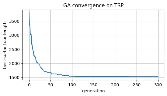
収束の様子は「各世代までの最良ツアー長（best-so-far）」で確認する．
最後に，得られた最良経路を可視化する．

# ==== 実行パラメータ ====
seed = 7
start_city = 0
num_cities = 30
pop_size = 120
generations = 300
crossover_prob = 0.9
mutation_prob = 0.08
elite_count = 4
tournament_k = 4


def initialize_problem(
    *,
    seed: int,
    num_cities: int,
    pop_size: int,
    start_city: int,
) -> tuple[np.random.Generator, np.ndarray, np.ndarray]:
    """都市座標と初期集団を生成し、始点固定の正規化を行う。"""
    rng = np.random.default_rng(seed)
    coords = random_city_coords(n=num_cities, xmax=300, ymax=300, rng=rng)
    population = initial_population(pop_size=pop_size, n=num_cities, rng=rng)
    population = normalize_population_start(population, start_city)
    return rng, coords, population


def run_experiment(
    *,
    coords: np.ndarray,
    population: np.ndarray,
    rng: np.random.Generator,
    generations: int,
    pop_size: int,
    crossover_prob: float,
    mutation_prob: float,
    elite_count: int,
    tournament_k: int,
    start_city: int,
) -> tuple[float, np.ndarray, np.ndarray, np.ndarray]:
    """GA を指定世代だけ実行し、世代ごとの最良値を記録する。"""
    best_length = np.inf
    best_route = population[0].copy()
    best_trace = np.empty(generations, dtype=np.float64)
    generation_best_lengths = np.empty(generations, dtype=np.float64)
    generation_best_routes = np.empty((generations, num_cities), dtype=np.int64)

    pop = population.copy()
    for t in range(generations):
        pop, _ = ga_tsp_one_generation(
            population=pop,
            coords=coords,
            rng=rng,
            pop_size=pop_size,
            crossover_prob=crossover_prob,
            mutation_prob=mutation_prob,
            elite_count=elite_count,
            tournament_k=tournament_k,
            start_city=start_city,
        )

        lengths = tour_lengths(pop, coords)
        idx = int(np.argmin(lengths))
        current_best = float(lengths[idx])
        current_route = normalize_route_start(pop[idx], start_city)

        generation_best_lengths[t] = current_best
        generation_best_routes[t] = current_route

        if current_best < best_length:
            best_length = current_best
            best_route = current_route.copy()

        best_trace[t] = best_length

    return best_length, best_route, best_trace, generation_best_lengths, generation_best_routes


def plot_convergence(best_trace: np.ndarray) -> None:
    """最良値の推移を可視化する。"""
    plt.figure(figsize=(6, 3))
    plt.plot(best_trace)
    plt.xlabel("generation")
    plt.ylabel("best-so-far tour length")
    plt.title("GA convergence on TSP")
    plt.grid(True)
    plt.show()


def build_animation(
    *,
    coords: np.ndarray,
    generation_best_lengths: np.ndarray,
    generation_best_routes: np.ndarray,
    generations: int,
    start_city: int,
):
    """世代ごとの最良個体をアニメーションとして構築する。"""
    from matplotlib.animation import FuncAnimation

    fig, ax = plt.subplots(figsize=(5, 5))
    ax.scatter(coords[:, 0], coords[:, 1], c="tab:blue", s=38, zorder=3)
    _annotate_city_ids(ax, coords)

    tour_arrows: list[FancyArrowPatch] = []

    def clear_tour_arrows() -> None:
        for p in tour_arrows:
            p.remove()
        tour_arrows.clear()

    (start_goal_marker,) = ax.plot(
        [], [], marker="o", color="tab:green", ms=8, zorder=4
    )
    start_goal_label = ax.annotate(
        "",
        xy=(0.0, 0.0),
        xytext=(8.0, 8.0),
        textcoords="offset points",
        color="tab:green",
        fontsize=10,
        fontweight="bold",
        zorder=6,
    )

    ax.set_xlabel("x")
    ax.set_ylabel("y")
    ax.set_aspect("equal", adjustable="box")

    x_min, y_min = coords.min(axis=0)
    x_max, y_max = coords.max(axis=0)
    pad_x = max(1.0, 0.05 * (x_max - x_min + 1e-9))
    pad_y = max(1.0, 0.05 * (y_max - y_min + 1e-9))
    ax.set_xlim(x_min - pad_x, x_max + pad_x)
    ax.set_ylim(y_min - pad_y, y_max + pad_y)

    sx, sy = coords[int(start_city)]

    def route_to_closed_points(route: np.ndarray) -> np.ndarray:
        ordered = normalize_route_start(route, start_city)
        pts = coords[ordered.astype(np.intp)]
        return np.vstack([pts, pts[0:1]])

    def init_anim() -> tuple:
        clear_tour_arrows()
        start_goal_marker.set_data([sx], [sy])
        start_goal_label.xy = (sx, sy)
        start_goal_label.set_text("START/GOAL")
        ax.set_title("generation = 0")
        return ()

    def update_anim(frame: int) -> tuple:
        route = generation_best_routes[frame]
        closed = route_to_closed_points(route)
        clear_tour_arrows()
        tour_arrows.extend(_draw_directed_tour(ax, closed))
        start_goal_marker.set_data([sx], [sy])
        start_goal_label.xy = (sx, sy)
        start_goal_label.set_text("START/GOAL")
        ax.set_title(
            f"generation = {frame + 1} / {generations}, "
            f"best = {generation_best_lengths[frame]:.3f}"
        )
        return ()

    ani = FuncAnimation(
        fig,
        update_anim,
        frames=generations,
        init_func=init_anim,
        interval=80,
        blit=False,
        repeat=True,
    )
    plt.close(fig)
    return ani


rng, coords, population = initialize_problem(
    seed=seed,
    num_cities=num_cities,
    pop_size=pop_size,
    start_city=start_city,
)

(
    best_length,
    best_route,
    best_trace,
    generation_best_lengths,
    generation_best_routes,
) = run_experiment(
    coords=coords,
    population=population,
    rng=rng,
    generations=generations,
    pop_size=pop_size,
    crossover_prob=crossover_prob,
    mutation_prob=mutation_prob,
    elite_count=elite_count,
    tournament_k=tournament_k,
    start_city=start_city,
)

print(f"best length = {best_length:.3f}")
print(f"best route  = {best_route.tolist()}")

assert np.array_equal(
    np.sort(best_route), np.arange(num_cities)
), "route is not a valid permutation"
assert int(best_route[0]) == start_city, "start city changed unexpectedly"

plot_convergence(best_trace)
ani = build_animation(
    coords=coords,
    generation_best_lengths=generation_best_lengths,
    generation_best_routes=generation_best_routes,
    generations=generations,
    start_city=start_city,
)

try:
    from IPython.display import HTML, display

    display(HTML(ani.to_jshtml()))
except Exception:
    plot_tour(
        best_route,
        coords,
        title=f"Best tour length = {best_length:.3f}",
        start_city=start_city,
    )

best length = 1517.079
best route  = [0, 11, 20, 17, 19, 16, 13, 8, 18, 7, 23, 10, 21, 27, 29, 28, 1, 2, 15, 6, 26, 12, 3, 4, 14, 25, 9, 22, 24, 5]

5. 実装のモジュール分割（推奨）¶

役割ごとに関数を分けると、コードの見通しがよく、課題や改良もしやすい。

役割	例となる関数名	内容
問題生成	`generator`	都市座標の生成、初期染色体（順列）集団 $P(0)$ の生成
評価	`evaluate`	各個体の $L(\pi)$ と適応度 $g_i$ の計算
選択	`selection`	選択操作（ roulette / fitness proportionate 等）、エリートの選出
交叉	`crossover`	交叉操作（ OX 等、 crossover rate 付き）
突然変異	`mutation`	突然変異操作（ swap 、 mutation rate 付き）
可視化	`show_route`	経路のプロット

以下は メインループ（main loop） の概形である（ $P(t)$ は世代 $t$ の 個体集団（population） ）。

初期化（都市・集団 P(0)）
各個体の適応度 g_i を計算
for t in range(T):
    P' = ルーレット選択(P(t), g)  # 適応度比例で親候補（例）
    P'' = 交叉(P', crossover_prob)
    P(t+1) = 突然変異(P'', mutation_prob) + エリート
    各個体の適応度 g_i を計算

6. パラメータの目安とチューニングの考え方¶

次のようなパラメータを変えて挙動を確かめるとよい（値は問題規模に応じて調整する）。

都市数 num （number of cities）、個体数 pop_num （population size）、世代数 generation_num （generations）
ルーレット選択を使う場合は 適応度のスケール （ $g_i$ の定義や フィットネススケーリング（fitness scaling） の有無）が結果に効く。トーナメント併用時は トーナメントサイズ（tournament size） など
エリート数（elite count） 、 交叉確率（crossover probability） 、 突然変異確率（mutation probability）

定性的には次を覚えておくとよい。

個体数が小さい と 多様性（diversity） が不足し、早い世代で悪い 局所解（local optimum） に張り付きやすい。
突然変異が小さすぎる と探索が停滞しやすい。 大きすぎる と良い順序が壊れやすい。
エリートを入れない と最良解が消えることがある。 大きすぎる と多様性が失われやすい。

7. 演習の進め方（目安）¶

7.1 まず設計を固める¶

TSP の 染色体 （順列）と目的関数 $L(\pi)$ 、 適応度 $g_i$ の対応を紙に書いて確認する。
binary ノート §2.2 の各ステップ（初期化→評価→選択→交叉→突然変異→世代交代）について、「入力は何か・出力は何か」を表にまとめる（§4章と対応づける）。

7.2 次に実装する¶

evaluate だけを先に動かし、ランダムな順列の距離分布を確かめる。
次に selection → crossover → mutation → メインループの順に足していく。
最後に最良距離の 世代ごとの推移 をプロットする（matplotlib）。

8. レポート課題¶

以下の2点を課題とする．

パラメータ実験
都市数 $n$ 、個体数、突然変異率のいずれかを変え、最終的な最良距離と収束の速さを比較する。
交叉の比較（発展）
順序交叉と、別の順列用交叉（PMX など）を1つ実装し、同条件で比較する。

課題１：パラメータ実験¶

変更点¶

...

コード¶

...

Ellipsis

考察¶

¶

課題２：交叉の比較¶

実装した交叉の説明とコード¶

...

考察¶

...

9. 参考資料¶

遺伝的アルゴリズム（立命館大学情報理工学部）
- 染色体・遺伝子・適応度、遺伝的操作（選択・交叉・突然変異）、個体集団の更新の流れなど、この資料の用語は主にここに沿っている。
遺伝的アルゴリズム（GA）巡回セールスマン問題 #Python（Qiita）
- Python による TSP×GA の実装例（ generator / evaluate / selection / crossover / mutation / 可視化などの分割の参考）。
- トーナメント選択＋エリートを用いている。記事の最終更新から年数が経過しているため、自分の環境で動作確認すること。

10. 確認問題¶

TSP の解を順列で表すとき、「制約」は何に対応しているか。
なぜ TSP では、ビット列の 一様交叉 のような単純な交叉がそのまま使いにくいか。
最小化の TSP で $L$ を小さくしたいとき、 適応度 $g_i$ をどのように定義すれば、参考資料の「大きいほど良い」選択と整合するか。
エリート主義を入れる利点と、入れすぎたときのリスクを述べよ。
GA で得られた解が最適解であると言えるか。根拠とともに述べよ。